Distributed Training Lexicon
Below contains 50 terms often used with Distributed Training, and a few visualizations made with Manim in the hopes to give you a quick reference to some of the terminology you may see online.
If you’d like to learn more, check out my course starting in September which will discuss all about this.
1. Parallelism Strategies
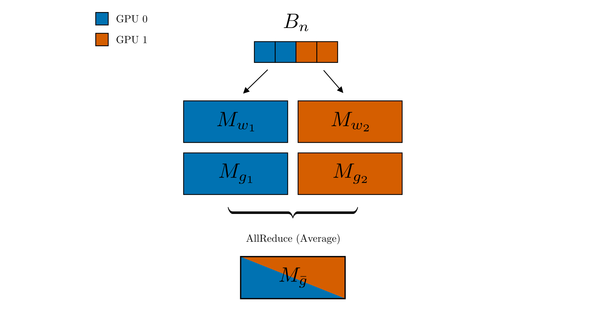
1.1 Data Parallelism
Data parallelism replicates the entire model on every GPU, partitions the training data across devices, and uses an all-reduce operation to average locally computed gradients after each mini-batch, ensuring synchronized replicas. It scales training by increasing the effective batch size with the number of devices but requires each GPU to hold the full model and incurs communication overhead proportional to model size. Frameworks like PyTorch DistributedDataParallelism automates the process, while techniques such as gradient accumulation, gradient compression, and lightweight optimizers are used to reduce communication costs.
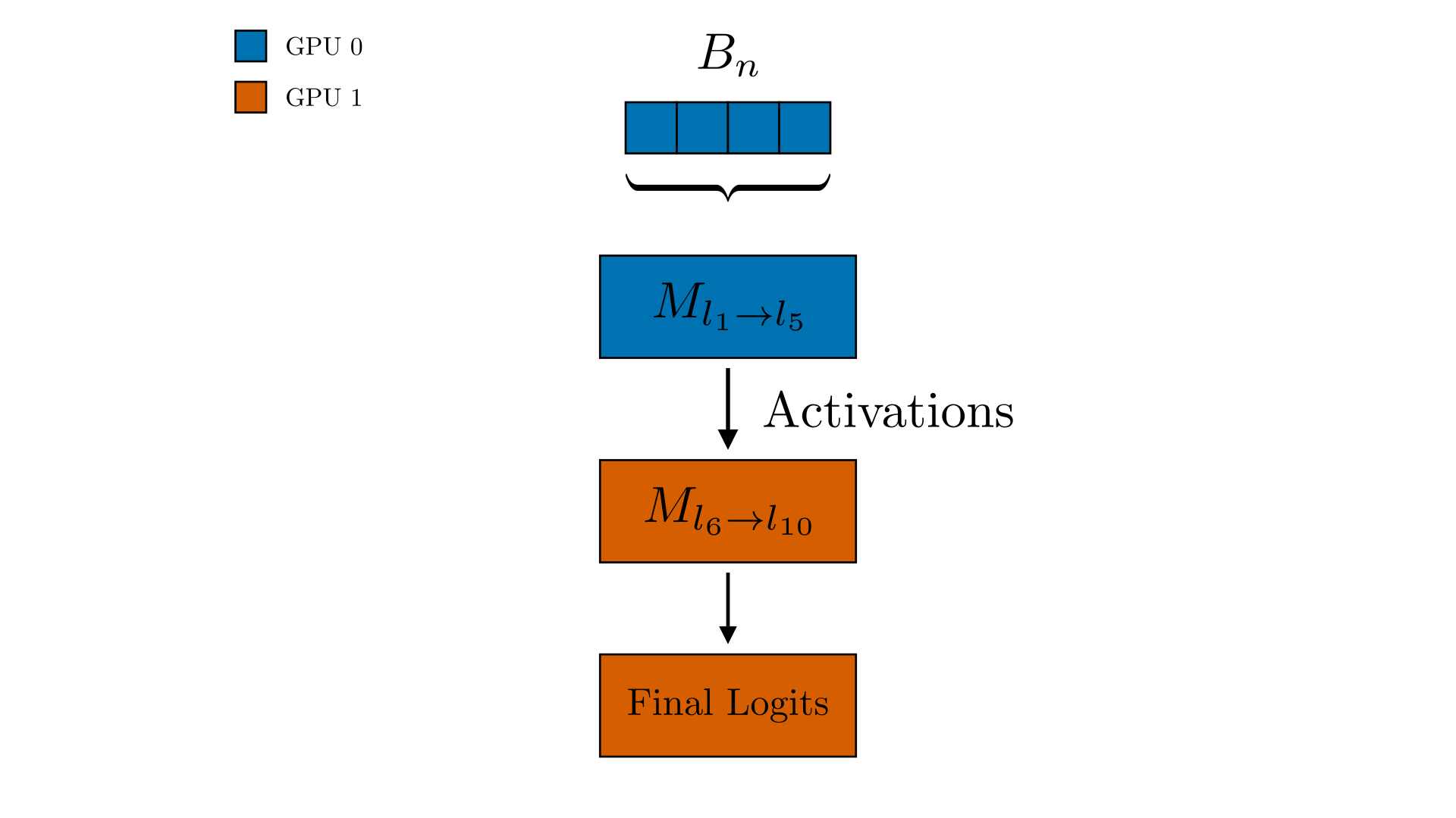
1.2 Model Parallelism
Model parallelism splits a model that exceeds single-GPU memory across devices, assigning distinct layers or operations to each so activations and gradients flow sequentially during forward and backward passes. By avoiding full-model replication it enables training of very large networks, but demands careful graph partitioning and introduces heavy inter-device communication that can idle GPUs unless mitigated with techniques such as pipeline parallelism.
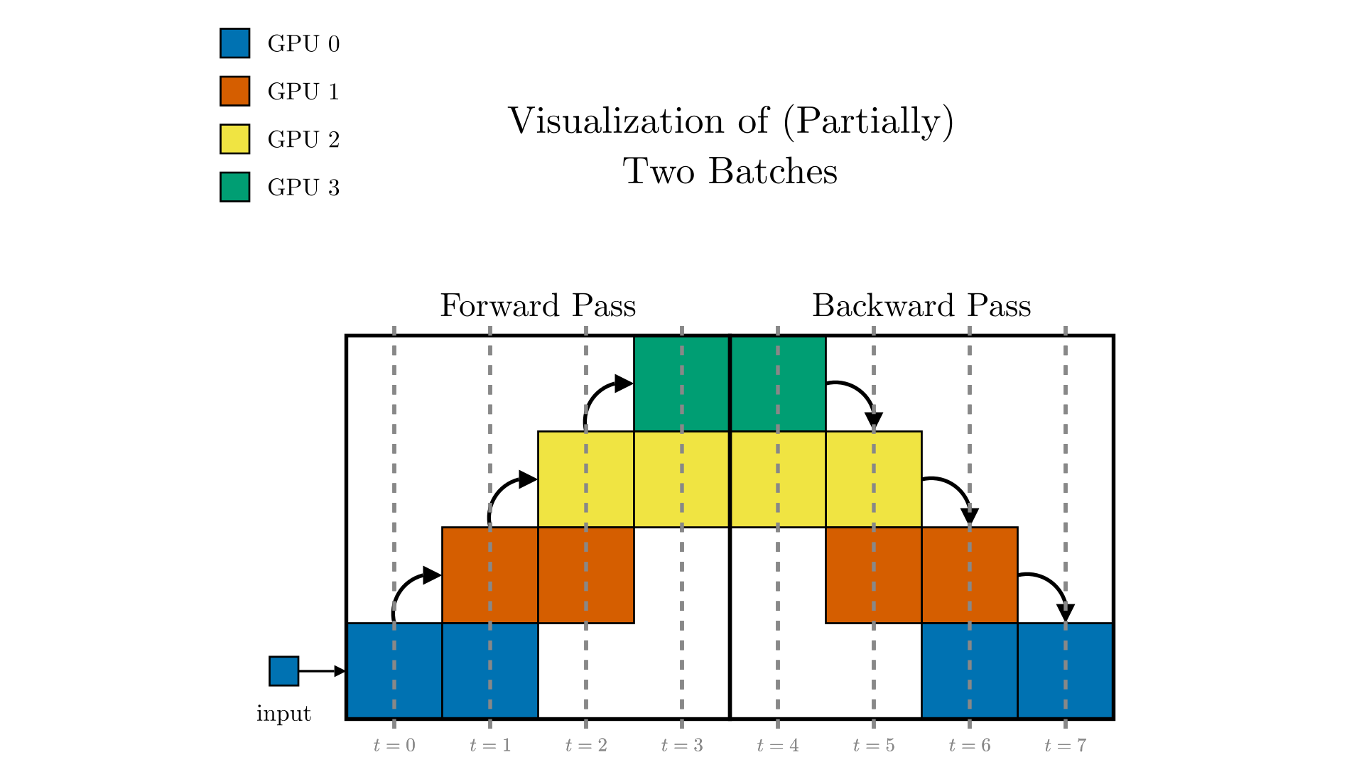
1.3 Pipeline Parallelism
Pipeline parallelism splits a model’s layers across devices and executes successive micro-batches in an interleaved fashion, letting one stage compute on micro-batch n+1 while another handles the backward pass for micro-batch n, thereby shrinking idle “bubble” time. Efficiency hinges on the number of micro-batches, balanced stage loads, and schedules such as 1F1B or interleaved 1F1B, which keep the pipeline full at the cost of communicating activations and gradients between stages.
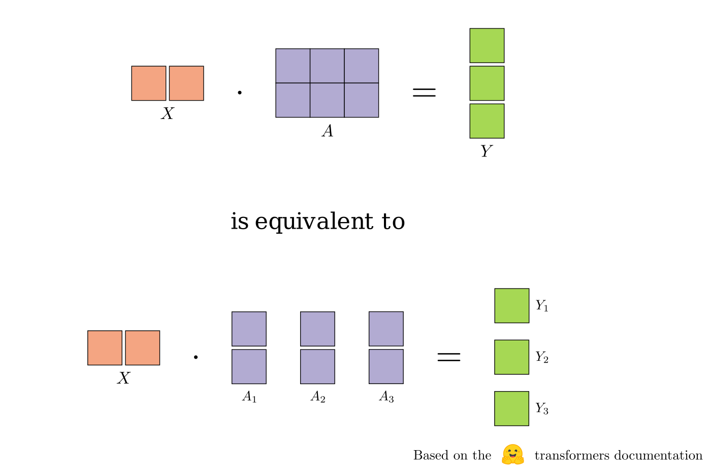
1.4 Tensor Parallelism
Tensor parallelism shards individual tensors (weights and activations) across GPUs so each device performs only part of a layer’s computation (e.g., splitting a large weight matrix by rows or columns), then uses collective operations such as all-reduce to merge partial results and maintain correctness. It’s needed for layers whose parameters exceed single-GPU memory and is best shown by Megatron-LM or nanotron’s transformer blocks, but its efficiency hinges on careful partitioning and fast communication of activations. Tensor parallelism is typically combined with data or pipeline parallelism to form hybrid schemes that scale to the largest models while balancing memory, compute, and network overhead.
1.5 Hybrid (2D) Parallelism
2D Parallelism is when you take two of the prior 3 parallelism techniques and combine them at once. Typically this is in the form of 2D Tensor Parallelism, where the model parallelism happens across horizontally and the data parallelism ocurs vertically.
1.6 3D Parallelism
3D Parallelism arranges all GPUs into a 3-D grid: tensor parallelism splits each layer across a few tightly-coupled GPUs inside one machine, pipeline parallelism assigns successive groups of layers to different machines in an assembly line, and data parallelism replicates that entire pipeline so every replica trains on its own slice of the data—letting trillion-parameter models fit into memory and keep every GPU busy. Typically this is accomplished with frameworks like Megatron-LM or nanotron.
2. Memory Optimization Techniques
2.2 ZeRO (Zero Redundancy Optimizer) - Stages 1, 2, 3
ZeRO is DeepSpeed’s set of optimizations that slices the model’s weights, gradients, and optimizer states across all GPUs so each device stores only a fraction; this staged partitioning slashes per-GPU memory and lets you train models far larger than the memory of any single GPU. Each of these are available in PyTorch’s FSDP using the proper configuration. The following table summarizes the key characteristics of ZeRO stages 1, 2, and 3:
| Feature | ZeRO-1 | ZeRO-2 | ZeRO-3 |
|---|---|---|---|
| Partitioned States | Optimizer States | Optimizer States, Gradients | Optimizer States, Gradients, Model Parameters |
| Memory Reduction | ~2–4× (vs. standard DP) | ~4–8× (vs. standard DP) | ~8–16× (vs. standard DP) |
| Communication | No additional overhead beyond standard DP (all-reduce for grads) | All-reduce for grads, reduce-scatter for gradient shards | All-gather for parameters, reduce-scatter for gradients |
| Key Benefit | Reduces optimizer state memory | Further reduces gradient memory | Maximizes memory savings by sharding parameters |
Table 1: Comparison of ZeRO Stages 1, 2, and 3
ZeRO Stage 1 (Optimizer State Partitioning): In this stage, the optimizer states (e.g., for the Adam optimizer, this includes the 32-bit weights, and the first and second moment estimates) are partitioned across the data parallel processes . Each process is responsible for updating only its partition of the optimizer states. This significantly reduces the memory required to store the optimizer states on each GPU, typically by a factor equal to the data parallelism degree. For example, if training with 8 GPUs in data parallel, each GPU would only store 1/8th of the optimizer states. During the optimizer step, each GPU updates its assigned portion of the parameters, and then an all-gather operation is performed to make the updated parameters available to all GPUs.
ZeRO Stage 2 (Gradient Partitioning): Building upon Stage 1, ZeRO Stage 2 also partitions the reduced 16-bit gradients across the data parallel processes . Each process retains only the gradients corresponding to its portion of the optimizer states (which were partitioned in Stage 1). This further reduces the memory footprint by eliminating the need to store the full set of gradients on each GPU. After the backward pass, a reduce-scatter operation is used to distribute and reduce the gradients to their respective owners. This stage effectively reduces the memory for gradients by the data parallelism degree.
ZeRO Stage 3 (Parameter Partitioning): In this most advanced stage, the 16-bit model parameters themselves are partitioned across the data parallel processes . ZeRO-3 automatically collects and partitions them as needed during the forward and backward passes. This means that at any given time, each GPU only holds a fraction of the model parameters. During the forward pass, if a GPU needs parameters it doesn’t own, it fetches them from the GPU that does own them (all-gather). Similarly, during the backward pass, gradients are computed for the local parameters, and then parameters might need to be gathered again for the next layer’s computation or for the optimizer step if it’s not fully sharded. This stage offers the most significant memory reduction for model parameters, also by a factor of the data parallelism degree.
ZeRO-3 also includes the “infinity offload engine” which, when combined, forms ZeRO-Infinity. This engine allows offloading optimizer states, gradients, and parameters to both CPU memory and NVMe memory, providing even larger memory savings and enabling the training of models with trillions of parameters . The communication overhead increases with each stage of ZeRO, so there’s a trade-off between memory reduction and communication cost. The choice of ZeRO stage depends on the model size, the number of GPUs, and the available inter-GPU bandwidth.
2.3 FSDP (Fully Sharded Data Parallel)
FSDP is PyTorch’s memory-saving upgrade to DDP: every GPU stores only a shard of the model’s parameters, gradients, and optimizer states; before each layer runs it uses all_gather to collect the full weights, then frees them again, and after the backward pass it uses reduce_scatter to average and shard the gradients. By wrapping layers with an auto_wrap_policy (or letting size_based_auto_wrap_policy do it) and optionally offloading shards to CPU, FSDP keeps GPU memory low enough to train models far larger than DDP can handle.
2.4 Activation Checkpointing (Gradient Checkpointing)
Activation checkpointing (also called gradient checkpointing) is PyTorch’s built-in way to train bigger models on the same GPU.
During the forward pass, instead of keeping every intermediate activation in memory, you wrap chosen layers with torch.utils.checkpoint.checkpoint.
PyTorch then stores only the inputs to that block and a small “recipe” to re-execute it later.
During the backward pass, the wrapped block’s activations are re-computed on-the-fly before the gradients are calculated.
This shrinks peak memory by roughly the inverse of the number of checkpoint segments, at the cost of one extra forward pass per segment. To use it, apply checkpoint (or checkpoint_sequential for a plain nn.Sequential) around memory-heavy sub-graphs—common choices are transformer blocks or large convolutional stacks.
FairScale and DeepSpeed wrap this mechanism for convenience, and it pairs naturally with FSDP to squeeze even larger models onto the same hardware.
The rule of thumb: checkpoint the layers whose activations dominate memory; each extra re-compute adds ~20 % per-step time, but the freed memory often lets you double the batch size or model width, yielding faster overall convergence.
2.5 CPU Offloading
CPU offloading moves model parameters, gradients, optimizer states, or even activations from GPU memory to the host’s much larger RAM (and optionally NVMe), letting you train bigger models or use larger batches when GPU memory is exhausted. Tools like DeepSpeed ZeRO-Infinity and PyTorch FSDP’s CPUOffload hook automatically handle the copying; they synchronize the transfers with ongoing GPU computation so the slower CPU memory doesn’t stall training.
2.6 NVMe Offloading
NVMe offloading treats fast SSDs as a third memory tier: ZeRO-Infinity (and similar libraries) can page infrequently-used model states or activations out of GPU/CPU memory onto multi-terabyte NVMe drives when even RAM is too small. Prefetching and pipelined transfers hide most of the added latency, so training trillion-parameter models remains feasible on modest-GPU clusters.
2.7 Mixed Precision Training (FP16, BF16)
Mixed Precision Training is where we keep some “chunk” of memory in a lower bit-precision than full (FP32). Typically we will end up with the model weights and gradients in half precision, while the optimizer states maintain full fp32 precision.
2.8 Gradient Accumulation
Gradient accumulation lets you train with a larger effective batch size than fits in GPU memory by running several small forward/backward passes, adding up their gradients, and applying the optimizer only after the desired number of micro-batches. In PyTorch this is as simple as calling loss.backward() for each micro-batch and then optimizer.step() after accum_steps iterations. When combined with pipeline or 3-D parallelism, the smaller micro-batches keep the pipeline full, reduce per-rank memory pressure, and still deliver the convergence behavior of the full global batch.
3. Communication Patterns and Collectives
3.1 All-Reduce (Ring All-Reduce, Hierarchical All-Reduce)
All-reduce is a collective operation that sums (or otherwise reduces) every corresponding element across all participating processes and returns the identical result to every rank, ensuring every GPU ends up with the same globally-aggregated buffer. It can be implemented efficiently via ring all-reduce, which pipelines reductions around a logical ring to minimize bandwidth, or via hierarchical all-reduce, which performs one reduction inside each node and a second across nodes to exploit fast intra-node links while limiting slower inter-node traffic.
3.2 All-Gather
All-gather is a collective operation in which every process supplies its own shard of data, and each process receives the full concatenation of all shards. In PyTorch and DeepSpeed, this is the workhorse behind ZeRO-3/FSDP: when a layer’s parameters are split across GPUs, an all_gather call momentarily reassembles the full tensor on every device so the layer can run, then the extra memory is released.
3.3 Broadcast
Broadcast is a collective operation in which a single root process sends an identical copy of its buffer to every other process; after the call, all ranks hold the same data. In distributed training it is typically used once at startup to distribute initial model weights or hyper-parameters from rank 0 to every worker, and occasionally later to propagate global updates such as newly averaged parameters.
3.4 Reduce-Scatter
Reduce-scatter is a collective operation in which every process contributes its own buffer, the buffers are element-wise reduced (usually summed) into one combined buffer, and that combined buffer is then split into equal chunks—each chunk sent to a different process—so every rank ends up holding only its unique shard of the reduced result. In PyTorch, this is the workhorse behind ZeRO-2/3: after each backward pass, reduce_scatter sums the gradients across GPUs and delivers just the slice each GPU needs to update its own parameter shard, avoiding the extra memory and traffic of a full all-reduce.
3.5 Gather
Gather is a collective operation where every process sends its buffer to a single root rank, and only that root receives the full concatenated result; all other ranks end with nothing. In PyTorch you call torch.distributed.gather(tensor, gather_list, dst=root_rank). gather_list is ignored on non-root ranks and on the root it becomes a list whose i-th element is the tensor from rank i. Typical uses are logging or diagnostics: after validation each worker sends its accuracy or loss to rank 0, which gathers them to compute and print global statistics.
3.6 Scatter
Scatter is a collective operation in which a root rank splits a single buffer into N equal chunks and sends one distinct chunk to every rank, including itself. After the call (torch.distributed.scatter(tensor, scatter_list, src=root_rank) in PyTorch) each process owns a unique slice of the original data. Typical uses are initial dataset partitioning or distributing embedding shards so every worker receives exactly the slice it will process.
3.7 Point-to-Point Communication
Point-to-Point (P2P) covers direct sends and receives between two ranks (send, recv, isend, irecv). In PyTorch you call torch.distributed.send(tensor, dst) and torch.distributed.recv(tensor, src); non-blocking variants (isend, irecv) let you overlap communication with compute. P2P is essential for pipeline parallelism, where adjacent stages exchange activations and gradients, and for custom model-parallel layouts that need fine-grained data flow.
3.8 Rendezvous
Rendezvous is the bootstrap step that lets every process discover the others and agree on roles (ranks, addresses). PyTorch’s torch.distributed.init_process_group uses a rendezvous URL (env://, tcp://, or etcd://) to register each worker and return a shared world-size and rank map. Without it, collective or P2P communication wouldn’t know where to send data.
4. Optimization and Training Techniques
4.1 DiLoCo (Distributed Low-Communication)
DiLoCo is a federated-style optimizer for geo-distributed LLM training. Each worker runs many local AdamW steps (e.g., 500) on its own data, then broadcasts a compact “pseudo-gradient” to a central outer optimizer (e.g., Nesterov momentum). This infrequent sync cuts cross-region traffic by two orders of magnitude, enabling training across continents on spotty links while maintaining convergence. OpenDiLoCo provides reference PyTorch code.
4.2 ZeRO-Infinity
ZeRO-Infinity extends ZeRO-3 to spill optimizer states, gradients, and even parameters to CPU RAM and NVMe SSDs, letting you train trillion-parameter models on modest-GPU clusters. Its infinity offload engine prefetches tiles back to GPU memory just-in-time, while memory-centric tiling splits large Linear layers so only a tile is resident during matmul. DeepSpeed exposes this via JSON flags ("offload_param": {"device": "nvme"}).
4.3 Elastic Training (Elastic Averaging SGD - EASGD)
Elastic training allows the job to add or drop workers on the fly without restarting. New workers pull the latest checkpoint (warm start) and resume with an EDT_PULL_WEIGHT_TIME_OUT grace window. IBM Watson ML Accelerator and ElasticFlow automate this, redistributing data and re-sharding parameters so total throughput scales with available GPUs.
4.4 Warm Start
Warm start initializes a new run—or a recovered worker—from a saved checkpoint (weights + optimizer state) instead of random weights. In PyTorch you call load_state_dict on rank 0 then broadcast with torch.distributed.broadcast_state. This cuts convergence time after pre-emption, node failure, or when fine-tuning a pre-trained backbone.
4.5 Gradient Compression
Gradient compression shrinks what crosses the wire via quantization (e.g., 32-bit → 8-bit), sparsification (top-k or block-wise), or low-rank approximations. DeepSpeed ships 1-bit Adam/LAMB optimizers that correct for compression noise with error feedback and momentum rescaling, often halving inter-node traffic with <0.1 % accuracy loss.
4.6 Quantization Aware Training (QAT)
QAT inserts fake-quantize ops into the forward and backward passes so the model learns to be robust to 8-bit or 4-bit inference. PyTorch’s torch.quantization.prepare_qat swaps layers, trains in FP32, then converts to INT8. QAT is usually the last fine-tuning step on a pre-trained, sharded model and can be done in parallel across ranks.
4.7 Overlapping Computation and Communication
Overlap hides collective latency by launching non-blocking communication (all_reduce, all_gather) while GPUs keep crunching the next micro-batch or layer. PyTorch DDP/FSDP use bucket gradients and CUDA streams to pipeline; DeepSpeed schedules ops with a compute-communication timeline. Effective overlap can reclaim 10-30 % of step time on high-latency networks.
4.8 Asynchronous Optimizers
Asynchronous optimizers let workers push gradients to a parameter server without waiting for stragglers, trading staleness for higher throughput. Variants include ASGD and EASGD, which use momentum and adaptive learning rates to dampen stale-gradient noise. They shine on spotty cloud VMs or when scaling beyond fast, homogeneous clusters.
4.9 Sparsity Optimization (Pruning)
Sparsity optimization removes weights whose magnitudes fall below a threshold or are deemed unimportant, reducing both memory and FLOPs. During distributed training, sparse gradients can be transmitted—only non-zero values and indices—slashing all-reduce volume. PyTorch’s torch.nn.utils.prune and DeepSpeed’s sparse optimizers automate pruning while maintaining convergence.
4.10 Smart Parameter Sharding
Smart sharding decides where to place each parameter shard based on bandwidth, compute load, and memory, not just round-robin. Frameworks like Alpa model the device mesh and schedule tensor-parallel shards on NVLink GPUs and data-parallel shards across InfiniBand links, cutting communication cost by up to 2× versus naive placement.
5. Scalability and Efficiency
5.1 Weak Scaling
Weak scaling keeps the work per GPU constant while increasing total GPUs and global batch size. Ideal behavior is constant iteration time: doubling GPUs and batch doubles throughput. In practice, communication and optimizer overhead cause sub-linear gains; frameworks therefore tune bucket sizes and overlap to stay as close to linear as possible.
5.2 Strong Scaling
Strong scaling fixes the total problem size (dataset and global batch) and adds GPUs to reduce wall-clock time per epoch. Perfect strong scaling halves time when you double GPUs. Diminishing returns kick in as communication dominates compute; techniques like gradient compression and smarter sharding push the scaling curve closer to ideal.
5.3 Synchronous Training
Synchronous training forces every worker to complete forward/backward passes and all-reduce gradients before the optimizer step. PyTorch DDP and TensorFlow MirroredStrategy implement this lockstep approach, ensuring deterministic updates but making the whole job wait for the slowest worker (straggler).
5.4 Asynchronous Training
Asynchronous training lets workers update the model via parameter servers without global barriers. Faster workers don’t stall, but gradients can be stale, hurting convergence. Parameter-server setups or decentralized gossip algorithms (e.g., SWARM) fall here; staleness-aware optimizers and bounded-delay strategies mitigate accuracy loss.
5.5 Time-to-Train (TTT)
TTT is the total wall-clock time from job launch until the model hits the target validation metric. It folds in compute, communication, checkpointing, and straggler delays. Tuning TTT is the ultimate objective of every distributed optimization: smaller batch, bigger model, faster network, overlap, compression—all trade-offs are evaluated against TTT.
5.6 Sample Throughput
Sample throughput (samples/sec or tokens/sec) measures how much data the cluster processes per second. It is the product of per-GPU batch size, number of GPUs, and iterations per second, minus communication overhead. Monitoring it reveals bottlenecks—slow data loading, congested all-reduce, or under-utilized GPUs.
5.7 Network Topology Awareness
Topology awareness maps parallel groups to the physical interconnect: tensor-parallel ranks on NVLink GPUs inside the same node, pipeline stages on InfiniBand, and data-parallel replicas across racks. Alpa and ElasticFlow use bandwidth cost models to place shards, cutting inter-node traffic and improving scaling by 10-50 %.
5.8 Heterogeneous Hardware Support
Heterogeneous support lets a single job mix GPUs of different generations, CPUs, or even TPUs. Systems like HALoS and SWARM adapt batch sizes and pipeline depth per device to keep faster GPUs busy and route extra work around stragglers, achieving near-linear scaling even when nodes differ in memory or FLOPS.
6. General Concepts
6.1 Node
A node is one physical or virtual server in the cluster—think “one box with 8 A100s and 1 TB RAM.” Nodes communicate over InfiniBand or Ethernet; node count and GPUs-per-node determine how you shard models and schedule collective ops.
6.2 Worker
A worker is a single process that owns one GPU (or CPU slice) and runs the training loop. In PyTorch each worker has a unique rank; workers exchange gradients or activations via NCCL, Gloo, or MPI.
6.3 Accelerator
An accelerator is any compute unit faster than a CPU for tensor math—most commonly GPUs (NVIDIA, AMD), TPUs (Google), or FPGAs. Distributed training revolves around how to keep hundreds of these accelerators busy and in sync.
6.4 Batch Size (Global, Local, Effective)
- Local batch size: samples processed by one GPU in one step.
- Global batch size: local × number of GPUs.
- Effective batch size: global × gradient-accumulation steps. Choosing these numbers balances memory, convergence, and throughput.
6.5 Checkpointing (Model Checkpointing)
Checkpointing periodically writes the model, optimizer, and RNG states to disk so you can resume after failure or evaluate intermediate checkpoints. In sharded training (FSDP/ZeRO) the checkpoint is gathered from all ranks before saving on rank 0.
6.6 Fault Tolerance
Fault tolerance lets the job survive node crashes or pre-emption by restarting from the latest checkpoint or re-sharding across remaining workers. Elastic training frameworks automatically detect heartbeats and relaunch failed workers.
6.7 Backend (Communication Backend)
The backend (NCCL, Gloo, MPI) is the low-level library that implements all_reduce, broadcast, etc. Picking NCCL on NVIDIA GPUs gives the fastest collective performance; Gloo or MPI is used for CPU clusters or mixed-vendor setups.
6.8 MPMD (Multiple Programs, Multiple Data)
MPMD means each rank can run different code and data—for example, one set of ranks acts as parameter servers while others are workers. PyTorch’s RPC or custom launchers support MPMD when roles are fundamentally asymmetric.
6.9 Gradient Bucket
A gradient bucket is a buffer that aggregates many small gradients into one large tensor before an all-reduce. In PyTorch DDP you set bucket_cap_mb; larger buckets amortize latency but may delay overlap.